Problem Statement
We are given the famous Iris dataset and have been asked to find the top 3 out 4 features that best help classify any data point into one of the 2 categories- Setosa and Versicolor.
Data and Problem Understanding
The dataset has 4 features, “sepal length”, “sepal width”, “petal height” and “petal width”, all in centimeters and 1 target column with 3 labels belonging to class of iris plant, “setosa”, “versicolor” and “virginica”. This dataset has a total of 150 data points and is one of the oldest and most popular classification datasets used. The data is evenly distributed among the 3 classes. One class is linearly separable from the other 2; the latter are NOT linearly separable from each other.
The problem statement is asking to find the best combination of 3 out of 4 features that help solve a binary classification task. In this particular example, we will be considering “setosa” and “versicolor” as the target labels. From the original dataset,all the data points belonging to “virginica” will be removed and thus leaving us with 100 data points to work with.
We will be training a simple perceptron for a certain number of epochs over 3 different combinations of the 4 features. Through this training we will visualise, which combination helps the perceptron learn faster and that particular combination will be the desired result for the problem statement.
Solution Approach
First let us define a class that cotains the required functions to implement a perceptron. This blog assumes that the reader is familiar with the conceptual knowledge of perceptron. To know more please checkout this blog or you could Google it up and would easily find explanation that suits you best.
# save as perceptron.py file
import numpy as np

class Perceptron(object):
   def __init__(self, rate = 0.01, niter = 10):
      self.rate = rate
      self.niter = niter

   def fit(self, X, y):
      """Fit training data
      X : Training vectors, X.shape : [#samples, #features]
      y : Target values, y.shape : [#samples]
      """

      # weights
      self.weight = np.zeros(1 + X.shape[1])

      # Number of misclassifications
      self.errors = []  # Number of misclassifications

      for i in range(self.niter):
         err = 0
         for xi, target in zip(X, y):
            delta_w = self.rate * (target - self.predict(xi))
            self.weight[1:] += delta_w * xi
            self.weight[0] += delta_w
            err += int(delta_w != 0.0)
         self.errors.append(err)

      return self

   def net_input(self, X):
      """Calculate net input"""
      return np.dot(X, self.weight[1:]) + self.weight[0]

   def predict(self, X):
      """Return class label after unit step"""
      return np.where(self.net_input(X) >= 0.0, 1, -1)
Now let us load all the required libraries and the Iris dataset.
import pandas as pd
import numpy as np
import matplotlib.pyplot as plt

from perceptron import Perceptron
from matplotlib.colors import ListedColormap

# 0.1 = learning rate , 10 = epochs
pn = Perceptron(0.001, 10)

df = pd.read_csv('https://archive.ics.uci.edu/ml/machine-learning-databases/iris/iris.data', header=None)
On running df.head() the first 5 rows of the dataset can be visualised. Let us the redefine the target column to make it a binary classification problem. We will be subsetting the first 100 data points as our new dataframe because on careful observation it can be found that the last 50 rows belong to the class “virginica”. After this we will need to label encode the target column so that it is perceivable by the perceptron. Versicolor is represented by 1 and Setosa by -1. Any combination of 2 integer values can be used.
# defining the target variable with only 2 classes
labels = df.iloc[0:100, 4].values
# 1 (Versicolor) and -1 (Setosa)
labels = np.where(labels == 'Iris-setosa', -1, 1)
We will now define the feature column. To do this we will create 3 groups of features such that all possible combination of 3 out of 4 are covered.
# defining feature columns
# feature1 has 1st 3 features
feature1 = df.iloc[0:100, [0,1,2]].values
# feature2 has 2nd 3 features
feature2 = df.iloc[0:100, [1,2,3]].values
# feature3 has last 2 and 1st features
feature3 = df.iloc[0:100, [2,3,0]].values

# different feature sets (feature1, feature2, feature3) will be used to identify which 3 combination of features gives the best result
Training the perceptron with defined learning rate and epochs on all the 3 feature sets and plotting the misclassifications for every epoch.
# training the perceptron model on feature1
pn.fit(feature1, labels)
# y coordinates
print("Number of misclassifications per epoch: ",pn.errors)
# plotting training graph
plt.plot(range(1, len(pn.errors) + 1), pn.errors, marker='o')
plt.xlabel('Epochs')
plt.ylabel('Number of misclassifications')
plt.title("FEATURE SET 1")
plt.show()
The result for the 3 feature sets are as follows:

Change in number of misclassifications as the perceptron fits the data for every epoch with the information from feature set 1.
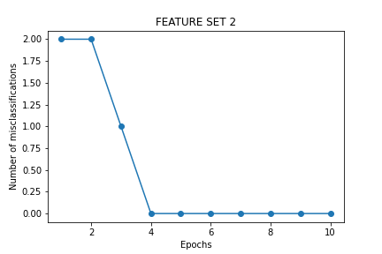
Change in number of misclassifications as the perceptron fits the data for every epoch with the information from feature set 2.

Change in number of misclassifications as the perceptron fits the data for every epoch with the information from feature set 3.
Observation
From the above 3 plots we can infer that when we have:
- feature set 1 (sepal length, sepal width and petal legth), the perceptrons learns the distribution at epoch number 6.
- feature set 2 (sepal width, petal legth and petal width), the perceptrons learns the distribution at epoch number 4.
- feature set 2 (petal legth, petal width and sepal length), the perceptrons learns the distribution at epoch number 5.
Conclusion
From this we can conclude that the combination of sepal width, petal legth and petal width out of the 4 features is enough to train the simple perceptron on binary classification problem.